The Birth of a Bot: Strategy Optimization - Strategy Building Basics (Part III)

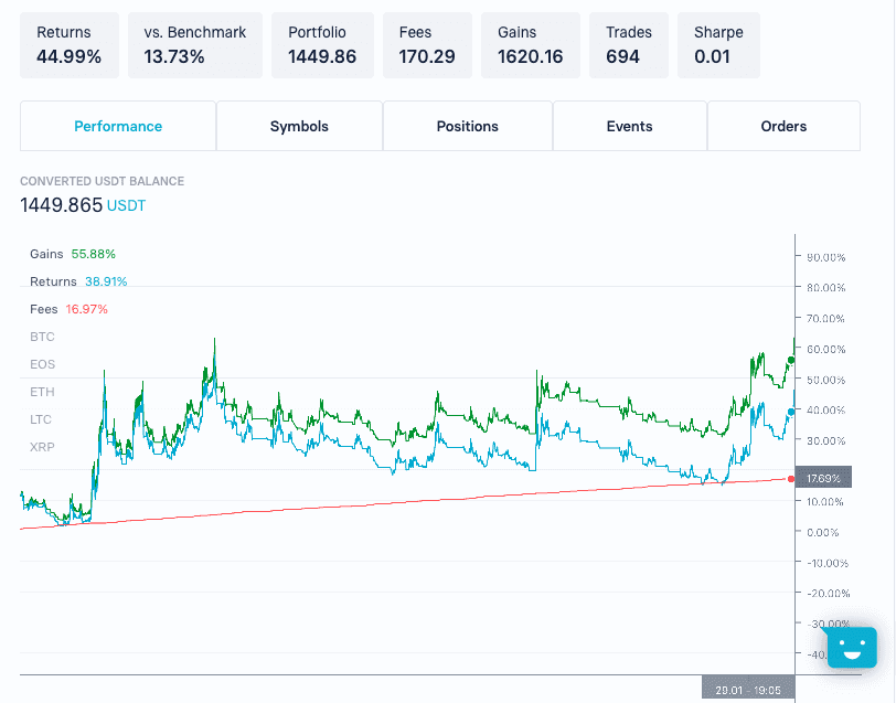
In the previous post we have created and backtested the base strategy for our multi-coin trend-following trading bot. We explained the necessary steps that need to be taken to arrive at a full grown live trading strategy. As a quick reminder, we summarise our defined base strategy for this post again:

A multi-coin trading strategy with an investment universe consisting of BTC, ETH, XRP, LTC and EOS. Our signal generator is the Exponential Moving Average Crossover on 1hr candles with a lookback period  of 20 and 40 hours.

In this post we investigate the choices that we have made for our base strategy in detail. We first take a closer look at our universe and how our signal generators work on asset individually. Second, we delve into optimal parameter selection to see how we can improve upon our base strategy. Last but not least, we give an outlook into further areas of potential improvement.

Investment Universe

For our universe, we have a few criteria that need to be fulfilled for each potential coin that we can trade:

- Tradability
- Applicability of the signal generators
- Diversification

Tradability

First of all, we must be able to trade a coin for it to be a valid candidate for our universe. It should moreover have existed before the start of our backtesting period (this is not necessarily required, we could also add coins that incepted during the backtesting window but for simplicity we will skip this possibility). Besides, each coin in our universe needs to have enough underlying liquidity for us to act upon our buy and sell signals. Please review our previous blog post for a more detailed discussion on the importance of liquidity.

Applicability of the signal generators

At this point we want to make sure that our signal generators (EMA Crossovers) can actually be employed on all individual assets in our universe. Furthermore applying these signal generators should be favourable - in terms of some performance metrics - for each asset in the universe. Admittedly, for some strategies it might not be straightforward to figure out if certain signals work for each asset by itself. However, for a trend-following strategy like ours in which the signal of one asset is independent of the signals for the other coins, this is easy! To compare the performance of signal generators on different assets we use the Sharpe Ratio. It is defined as the average return earned in excess of the risk-free rate per unit of volatility. It gives us a measure of profitability per unit of risk taken on.

Additionally to visualising only one Sharpe Ratio for our signal generators per asset we use a grid of parameters for both the short and long lookback periods. This way we get an even clearer picture on how our signal generators with a given set of parameters vary in performance for each asset. To get our parameter grid we take the short lookback period from 2 to 24hr and for the long lookback period from 4 to 48hr (we don't run the test on parameter combinations where the long parameter is shorter than the short one). Once we have obtained all Sharpe Ratios for the parameter combinations, we can plot the result on a surface.

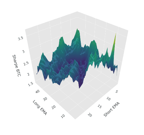
Ideally, what we would like to see here is a positive Sharpe Ratio that is similar across all parameter combinations. This would make it likely that our strategy is actually capturing trends independently from the parametrisation instead of just overfitting a backtest. When looking at the sample plot for BTC, we can see that all the results are positive, which is an excellent sign. We can also see that the maximum is a spike at the 4hr/8hr parameter combination. While it may be tempting to use these parameters, we can see from the plot that the Sharpe Ratio drops off significantly when moving only 1hr away. Generally, it is best to avoid obvious overfitted parameter combinations like that unless there is a compelling fundamental reason for this specific combination to work.

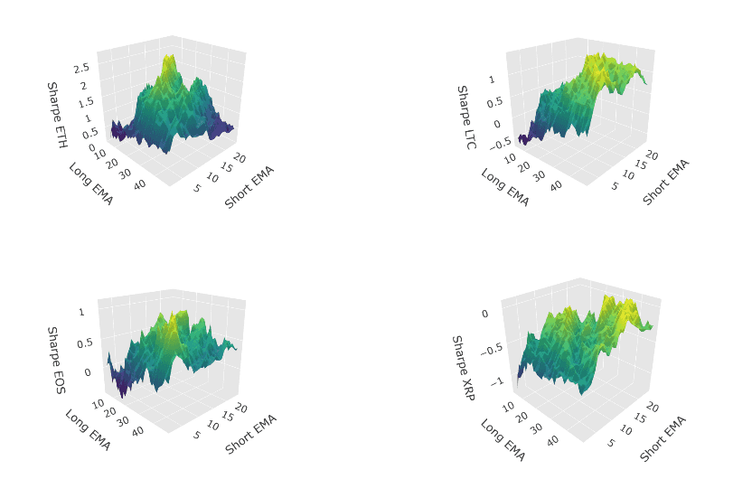
Upon inspection of the other four assets, we can see that they all display a positive Sharp Ratio except XRP! For this coin, almost all parameter combinations return a negative Sharpe Ratio! This means that on average we expect our signal generator to yield a negative return per unit of risk taken. Due to this unfavourable result we immediately remove XRP from our universe.

Diversification

Now that we have analysed all coins individually we are interested to see how our investment capital is spread among different coins over time. It is of no use if we have 20 different coins in our universe but they all produce the same signals. In that case, the most optimal solution would be to trade only one coin. What we want is that our individual signals display a low correlation, providing us with a diversified return profile and a smoother, more consistent equity curve.

The following chart displays our capital allocation in our remaining four coins over the backtesting period. This chart displays the percentage allocation in each asset across time. With this graphical representation we aim to get an overview about which assets we are invested in at different points in time.

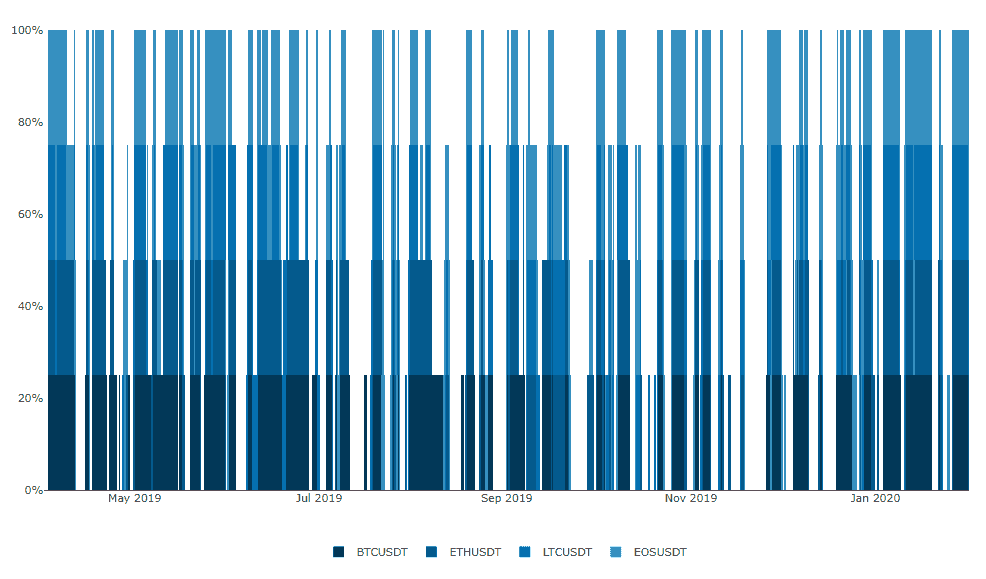
Although our signals agree a lot of the time (points in time with 100% investment), we can see that there is clearly enough diversification in the signals to keep all four remaining coins in our universe. In fact, the average total allocation over the backtesting period is 50.37%.

Now that we have adjusted our universe, let's take a look how our original 20hr/40hr parameter setting performs over the backesting period.

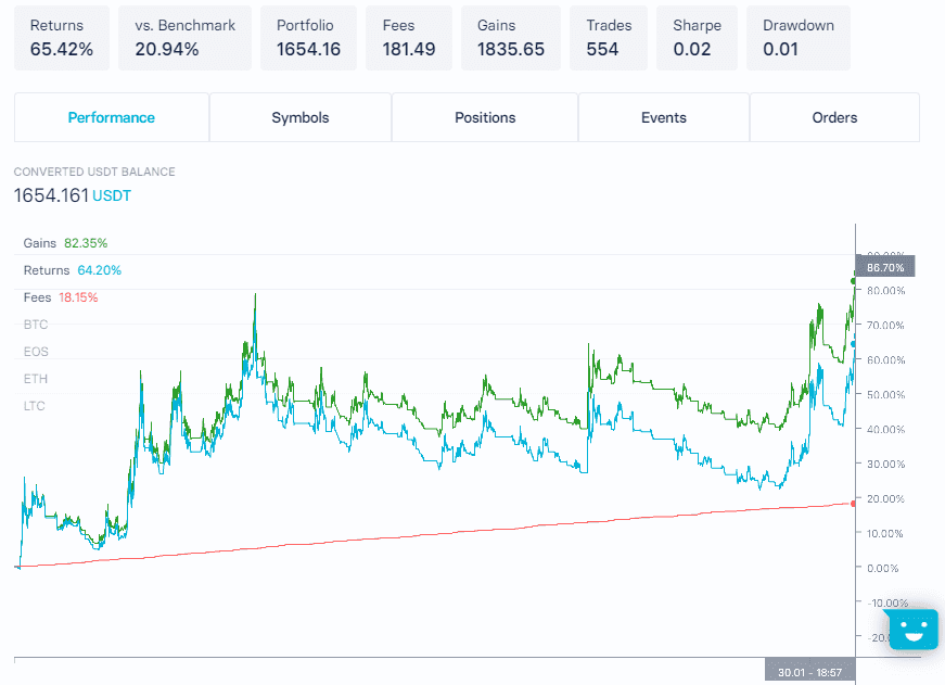
That is a quite significant improvement already! The return of our strategy is now 65.42% (vs 44.99% before) and we outperform the benchmark (which only consists of the 4 remaining coins) by 20.94%!

Parameters

After adjusting the universe we will now take a look at the specific parameters of this multi-coin bot. We have already seen that our backtest results improved quite dramatically after removing one coin while keeping our 20hr/40hr lookback periods untouched. But what can we achieve once we optimize those? Below we see the result of the same surface parameter optimization output that we already used in the universe selection.

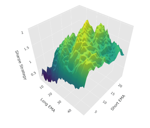
We can see that the results of the strategy do not work very well if both parameters are relatively short. When both parameters are on the longer end of our ranges (such as the 20hr/40hr combination), we can see that the strategy performs decent, but not as good as in the range in between. We have a maximum result on the 19hr/21hr combination, but all combinations on the "plateau" in the middle of the surface provide viable parametrisations. Let's have a look how the 10hr/30hr combination performs.

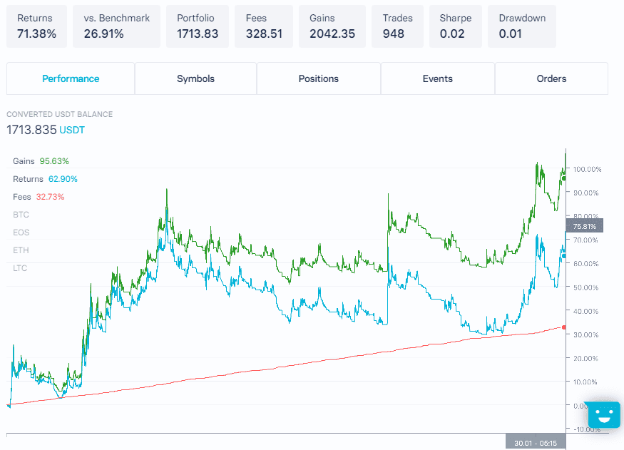
As expected, this provides an improvement yet again, another 6% increase in returns. What is immediately obvious from the result above is that not only does our return increase, but also the number of trades. We would have traded almost twice as much using this parametrisation. Excluding fees, the parameter change would have netted us a 20% increase in returns! This should serve as a reminder to never forget testing your strategy including the impact of trading costs.

There is no guide that can help you pick a "correct" parameter combination from our suitable set of combinations. You could argue that a "logical" choice would be 12hr/24hr as the number of hours has a specific meaning. You could also argue that this reasoning is completely arbitrary. In reality, you would use an ensemble strategy (closely related to ensemble learning), a combination of sub-strategies which signals are aggregated into an overall strategy. Simplified, you would use many different sets of parameters (preferably the ones that lie on the plateau of the surface) and average the resulting weights every time you are about to make a trade. This greatly reduces the potential of overfitting of your strategy and can increase the likelihood of continued performance when live trading. Ensemble strategies are coming to the Trality Rule Builder soon!

Out-of-Sample Testing

After looking at how to optimize the original strategy, let's check now how it would have performed out of sample. In correspondence to machine learning terminology this would be our test set. It is important to design and optimize your strategy using the in-sample period (the training set) and validate your strategy using the out of sample period.

We use the same four coins (BTC, ETH, LTC & EOS) as in our universe and use the 10hr/30hr parameter combination. We test the strategy between 2020-02-01 and 2020-07-14.

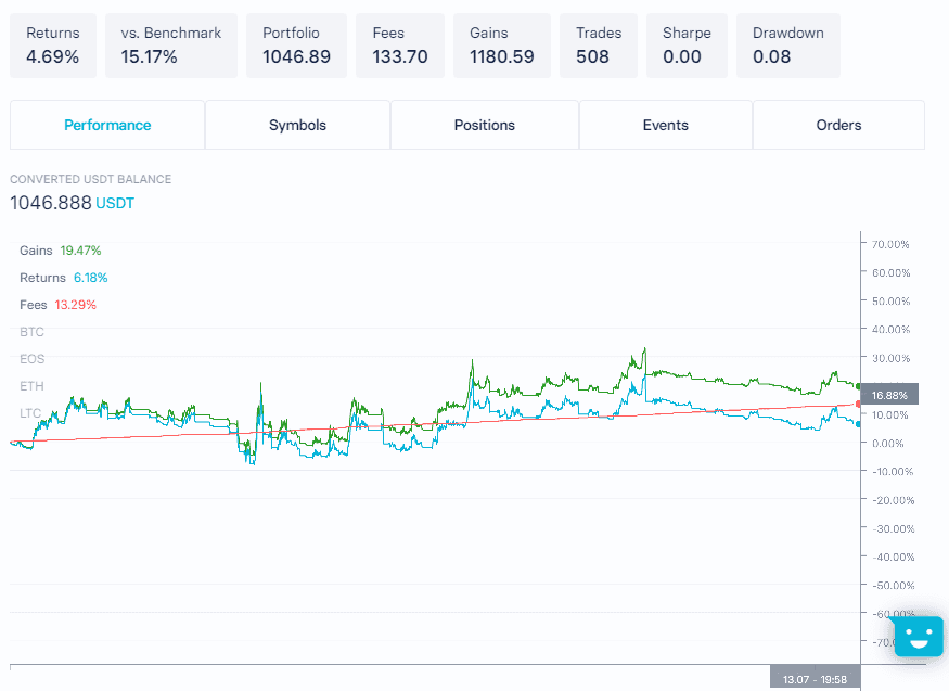
That looks promising! The strategy continued to perform even out of sample, and while the return is "only" 4.69%, we outperformed the benchmark by 15.17%! We can also see that the strategy seems to start to deteriorate at the end of the out-of-sample window. Strategy decay, it's effects and potential counter measures will be the topic of a future post here on the Trality Blog.

Outlook

The observant reader will have realised that we have left out some areas of improvement of our strategy. For example, we always assumed that our strategy weights are equally split between the coins in the universe. One could for example apply Risk-Parity weighting (allocating to the coins in such a way that their contribution to the overall risk of the strategy is equal).

Furthermore, the parameter settings for the EMA Crossover can become dependent on the general market volatility and require a combination that reacts faster or slower to changes (you can experiment yourself and find out if a combination of very short EMAs prevent the strategy decay towards the end of our out-of-sample test?). Lastly, our strategy only takes long positions. What if we would take short positions in our universe instead of simply closing the position?

All these are possible additions and tweaks to the strategy are  features of  our intuitive Rule Builder!

You can build the exact strategy we have detailed in this blog post, make changes and run backtests with our powerful backtester within one seamless ecosystem.

Get started automating your strategy and benefitting from the advantages of emotionless trading right now.

Stefan is a quant with more than 6 years experience in the finance industry. He currently holds the role of Director Risk Management & Analytics at an independent investment manager specialising in insurance investments for institutional clients. In his free time he has been developing and implementing algorithmic trading strategies across multiple asset classes for 7 years.