Finding the Best Strategy Parameters: An Introduction to Optimization Algorithms

Throughout the process of building your trading strategy, your underlying goal is to maximize your bot's profitability. In order to achieve this, you look for the best piece of code through a process of trial and error and guided by the results of the backtester. If you are quite confident that the general idea behind your strategy is sound, then you try to improve it by applying small changes and exploring different variations of it.

You probably already know that fine-tuning a strategy can be extremely time-consuming, especially if you want to explore many alternative settings (and the execution of the backtest is not instantaneous). Also, these changes often consist in tweaking some numerical parameters.

What you are doing is known as optimization and the good news is that, in several cases, it can be automated!

In this article, we will dive into optimization and how it can be applied to trading strategies. As we'll see, optimization will improve your bot by allowing it to leverage the power of data.

Strategy Optimization

Before talking about optimization, we have to introduce parameters and parametric strategies. Parameters are basically variables in a strategy whose values are not predefined. For example, the strategy

(S1) “Buy and hold 100$ of BTC when EMA(period₁) > EMA(period₂), close the position otherwise” is a parametric strategy that depends on two parameters: period1 and period2.

Applying this strategy to historical data (i.e., backtesting) will allow us to calculate different performance measures (e.g., PnL and Sharpe ratio).

Now the question is:

(Q1) Given a parametric strategy, which parameters' values will make my strategy profitable? Which ones are the best?

That's what we will attempt to answer, but this is a difficult question. Let's ask another question first:

(Q2) Given a parametric strategy and a certain period of time in the past, which parameters' values resulted in the best performance?

Question Q2 more closely resembles the kind of problem mathematical optimization tries to solve. We have a function f(•) and we want to find the input x from a certain set of alternatives such that f(x) is maximized or minimized. In our case, f(•) is the performance of a parametric strategy executed on a given period of time as a function of its parameters x. The performance could be any descriptive metric, the total return or Sharpe ratio, for example.

Going back to our previous example, the optimization problem could be stated in this way:

"Find values for period₁ and period₂ between 1h and 60 days that maximize the total return of strategy S1"

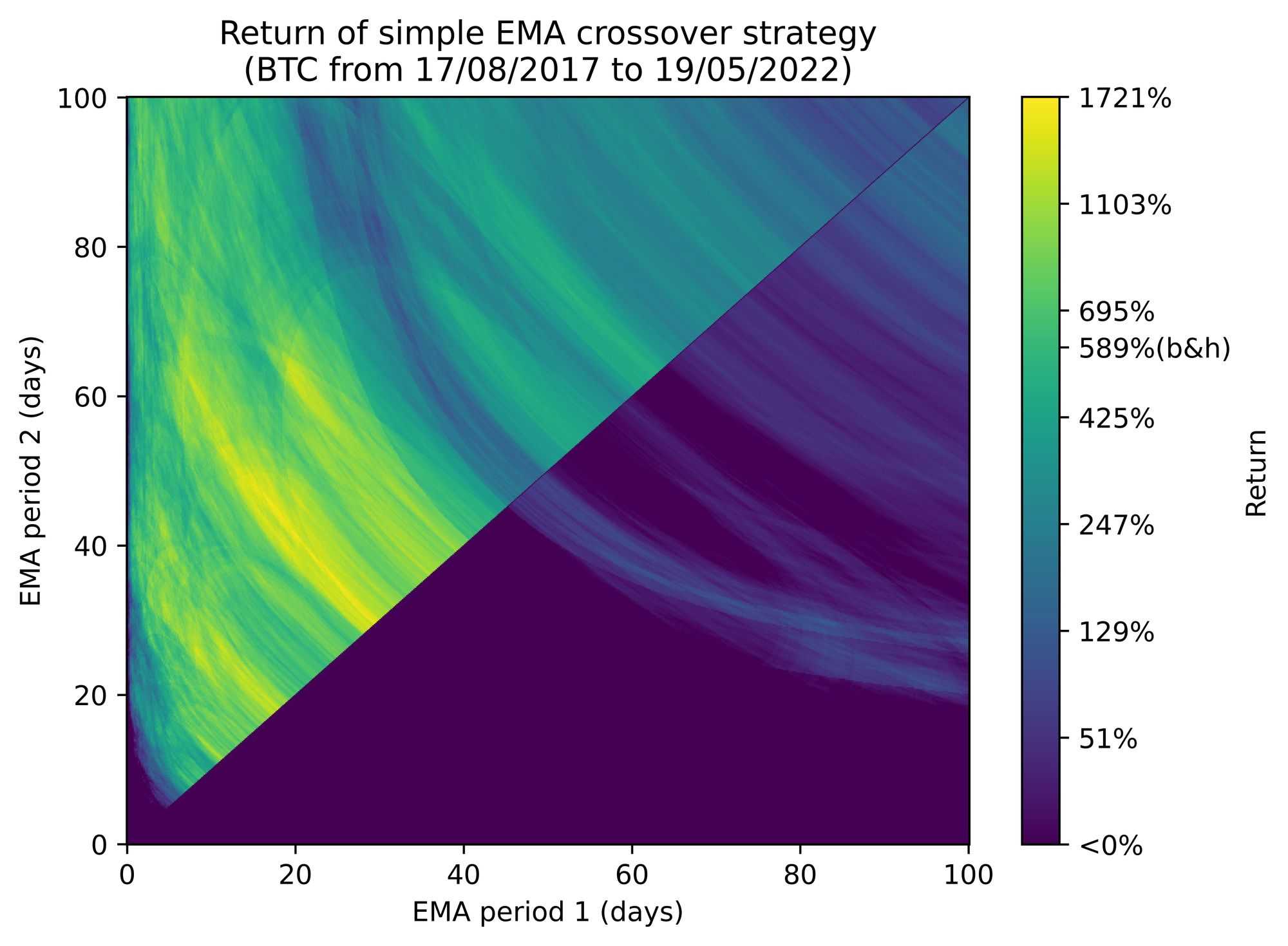
The following graph shows how the total return of strategy S1 looks like as a function of its two parameters:

We can also observe how the performance landscape changes in different scenarios:

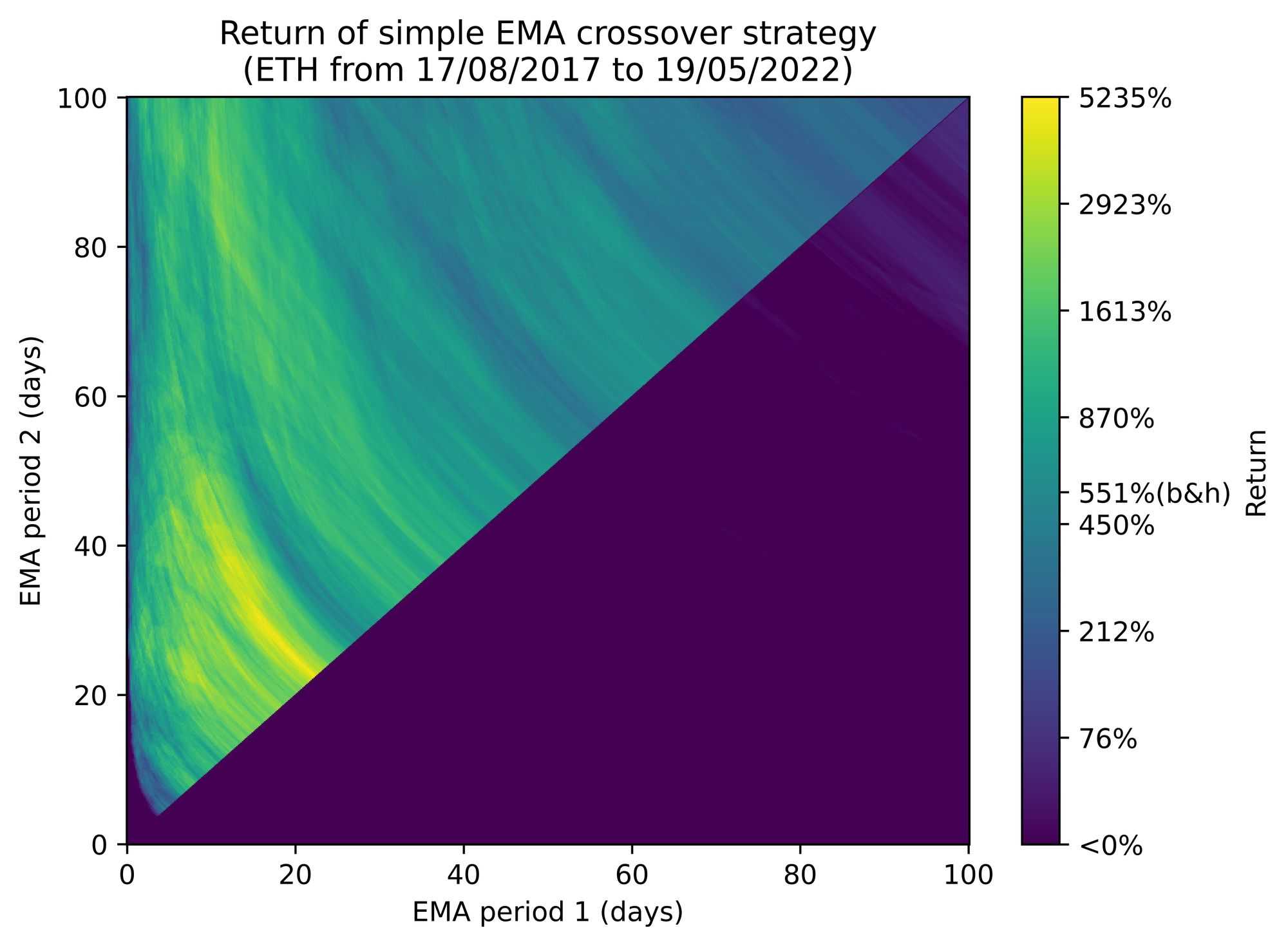
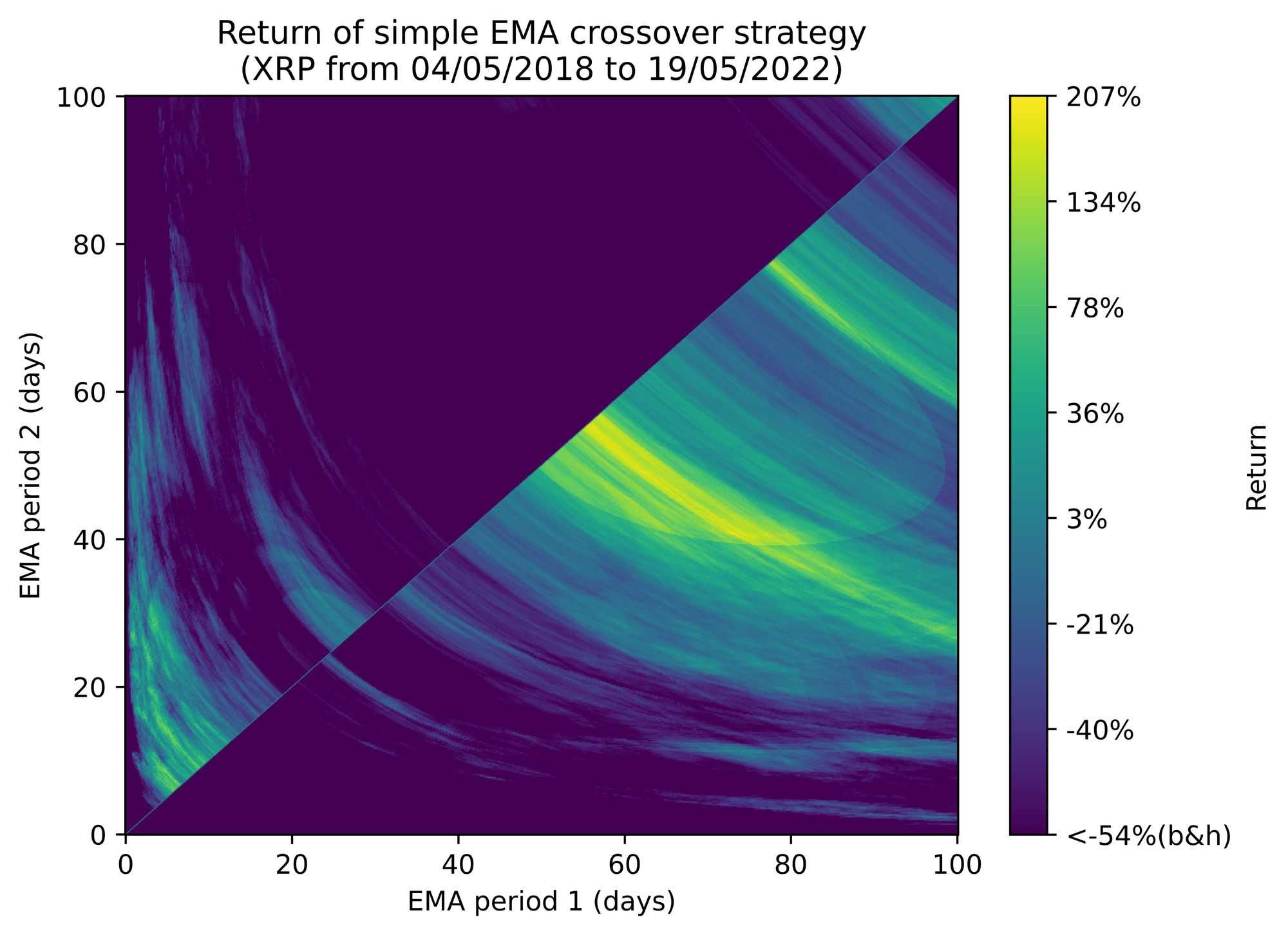
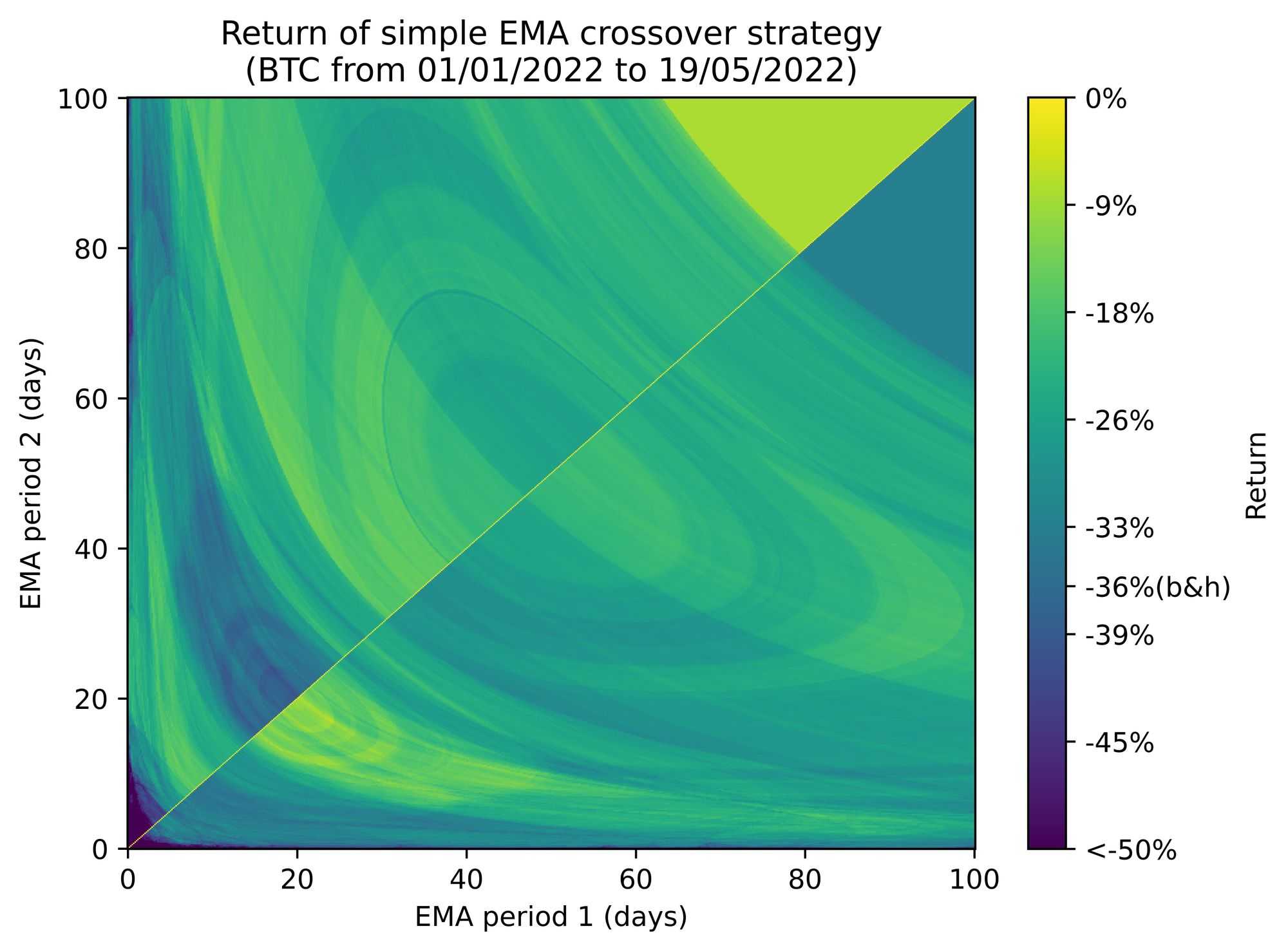
In the experiments above we can see that for BTC our solution, the optimum, is approximately at period₁=17 days and period₂=46 days for which we get a log₂ return of ≈ 4.

In order to generate these plots, we simply calculated a lot of combinations for the two parameters (360,000!), an unfeasible approach in most cases, where evaluating one point is very time-consuming or when there are too many parameters.

Therefore, we need to search for solutions in the parameter space in a smarter way. This challenge is tackled by advanced optimizers, which are optimization algorithms that try to find good solutions in a restricted amount of time or number of evaluations of the objective function.

Optimizers

Countless optimization algorithms have been developed, many of which are popular and available in scientific libraries like Scipy. This flourishing variety is partially due to the fact that optimizers are specialized in solving particular classes of problems that may differ in some fundamental characteristics.

Local and global optimization

There are problems where one can be satisfied with finding a local optimum without the guarantee that it’s also a global optimum. A local optimum is a value for the input for which the objective function is better than any other point in the immediate neighborhood. A global optimum, on the other hand, is a value for which the objective function has its best value with respect to the whole input domain.

An example of a local optimizer is a plain gradient descent, which consists of performing steps in the direction of local improvement of the function.

An example of a global optimizer is simulated annealing, where, without going into too much detail, random jumps from the current solution are performed in order to improve it.

Availability of Gradient Information

A differentiable function f(•) can be built such that given an input x and the value of the function f(x), it's possible to extract the gradient of f(•) at x, ∇f(x), without any additional evaluation of f(•).

The gradient information is really valuable since it tells us in which direction the function is going to improve independently of the number of parameters! This is a game changer and it's behind the enormous success of neural networks (here the computation of the gradient is known as back-propagation) in which the number of parameters can also be in the order of billions.

For example, let's say we have a function of two variables, f(•, •), and we want to evaluate it at the point (x₁=1,  x₂=3). We get f(1, 3)=2.5 and also ∇f(1, 3)=(x₁=-2, x₂=+1.5). This means that the function f(•, •) is going to increase if we perform a small step from (x₁=1, x₂=3) in the (x₁=-2, x₂=+1.5) direction, for instance (x₁=1 - 2 * 0.01, x₂=3 + 1.5 * 0.01).

Optimizers that exploit gradient information are often called gradient-based. Gradient descent is a basic example of this class of optimizers.

The setting where gradient information is not available is called gradient-free optimization. Gradient-free optimization is a quite different game; the objective function is more similar to a black box and often these algorithms struggle when dealing with a large number of parameters. Simulated annealing is an example of gradient-free optimization.

Another characteristic that could be considered is the smoothness of the objective function, i.e., if there are jumps in the function. While smoothness is a requirement in gradient-based optimization (otherwise it wouldn't be possible to calculate the gradient), it's not strictly necessary in gradient-free optimization. Nevertheless, it deserves attention since there are optimizers that rely on an empirical approximation of the gradient in order to determine the best direction to follow. This approximation will fail with non-smooth functions.

Picking the Right Optimizer for Trading Strategies

We’ve already seen how different problems require different optimizers, but which ones are best-suited to parametric trading strategies?

We can already make three assumptions:

1. We need a global optimizer, since there could be many unsatisfactory local optima and we want the optimizer to be able to reach the global optimum. However, local optimization can still be very useful in combination with global optimization.
2. We can safely say that we are dealing with gradient-free optimization. Building a parametric trading strategy differentiable with respect to its parameters is not impossible, but it would require special care and it would involve several limitations to the strategy itself. For example, let's consider the total return of the parametric strategy S1 as an objective function f(period₁, period₂). This function is not expressed as a composition of simple, differentiable functions with known derivatives, so one cannot calculate the gradient. Also this implies that there is no guarantee it's actually differentiable.
3. Non-smooth dependency of a strategy on its parameters is quite common, so it's safer to reject the smoothness assumption. For example, whenever a trade is triggered by a condition that depends on a real valued parameter, the trade is either executed or not; there is no middle way, which constitutes non-smoothness.

There are several optimizers that comply with these conditions, with some examples including grid search, Bayesian optimization, simulated annealing, particle swarm, evolutionary algorithms, and differential evolution. In the next sections, we will discuss a couple of these optimizers, which represent a good starting point.

Grid Search

Grid search is the most basic global optimization method. It works by evaluating the function in every point of a multidimensional grid and finally taking the best result. It’s also called "brute force optimization" since one simply tries every combination of some set of possible values for each parameter.

Let’s look at an example:

Imagine a trading strategy represented by the function f(•,•), which depends on the parameters p₁ and p₂, both real numbers belonging to the [0, 24] interval.

We build the grid of points by taking 5 equispaced values for each parameter and then combining them:

p₁ ∈ {0, 6, 12, 18, 24}

p₂ ∈ {0, 6, 12, 18, 24}

So we evaluate the function f at any combination of these values of p₁ and p₂: f(p₁=0, p₂=0), f(p₁=6, p₂=0), …

This is how grid search looks when applied to our EMA crossover example:

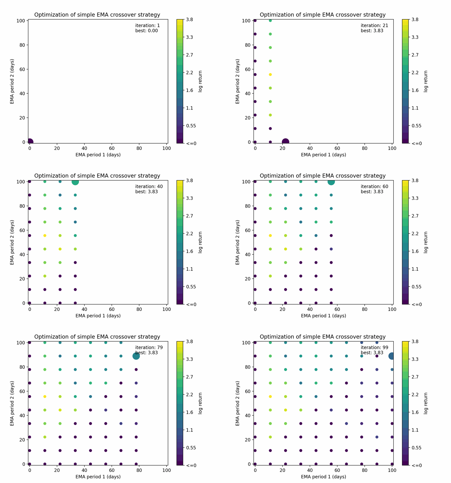
The rationale is to explore the parameter space in a uniform way with a limit of n guesses. Despite being a quite simplistic approach, it’s still valuable when there is absolutely no assumption about the objective function.

Bayesian Optimization

Bayesian optimization is a quite sophisticated approach in comparison with grid search, but its logic is still more straightforward than many other optimizers.

Bayesian optimization can be summarized by the following steps:

1. Fit a probabilistic model f_model(•) of f: x → f(x) using the set of already evaluated points {(x_i, f(x_i))}. The model f_model(•) maps every input x to a distribution of possible output values.
2. Select the point x_guess that correspond to the distribution f_model(x) that is expected to give the best improvement over the current best value.
3. Evaluate f(x_guess) and reiterate from 2.

This is Bayesian optimization in a nutshell, but let’s dive into the details.

First, suppose we want to maximize the objective function f(•) and we already start with a set of evaluated points {(x_i, f(x_i))} (we can randomly sample a few at the beginning).

The fitted probabilistic model is usually a Gaussian process. Gaussian processes are machine learning models that associate to each point x of the input space a normal distribution N(μ(x), σ(x)) as an estimate of f(•). The functions μ(•) and σ(•) are what is fitted by the model. It works roughly similar to a nearest neighbor model: μ(x) is close to f(•) of evaluated points close to x, σ(x) gets larger as x is far from any other point. So basically the assumption of Gaussian processes is that you expect f(x) of a point x to be close to the f(•) of points close to x, and your uncertainty increases as x is far from other evaluated points. Pretty reasonable, right?

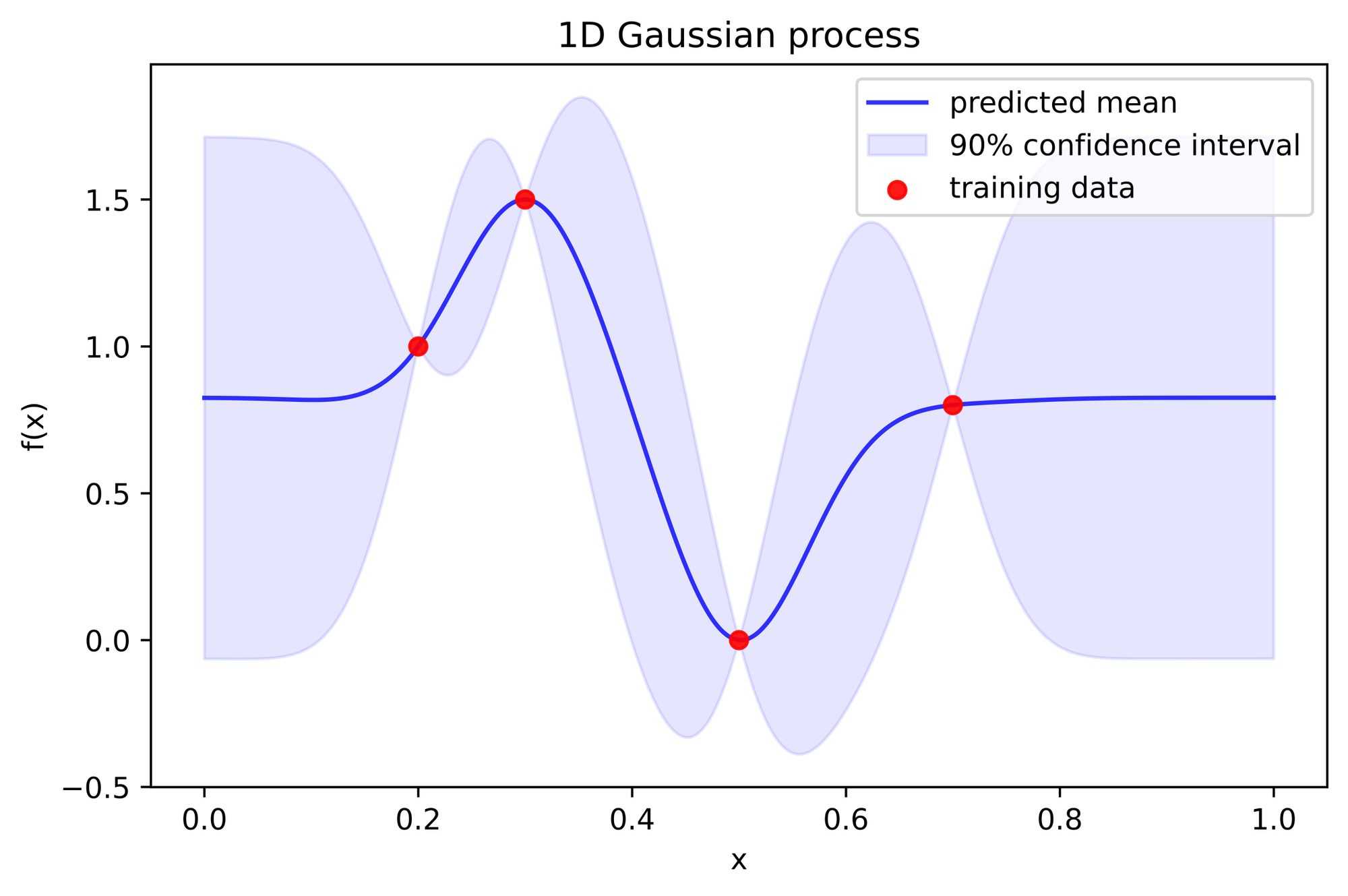
Now that we have a model f_model(•) that estimates f(•), we have a clearer picture of where to choose the next point to evaluate. We want to choose the x such that f_model(x) has a large expected value since we are doing maximization, but also large uncertainty since we want the potential improvement to be large.

For example, if the current maximum is 2, would you rather choose to evaluate f(•) at a where f(a) = N(μ=1.8, σ=5) or at b where f(b) = N(μ=1.9, σ=0.1)?

The first alternative looks better. Moreover, a common criterion is to pick x that maximizes the expected improvement over the current maximum. The chosen criterion is called acquisition function and it tells us how convenient it is to evaluate a certain point. So, given an acquisition function g(•), what we finally will choose is the x_guess such that g(f_model(x_guess)) is the best.

Now we ended up with a different optimization problem, but this is much easier since g(f_model(•)) is fast to evaluate (much faster than f(•)), smooth, and the gradient is available. Here we can solve this with any global optimizer (also the ones that need to perform a lot of function evaluations).

Let’s see how Bayesian optimization behaves with our EMA crossover example:

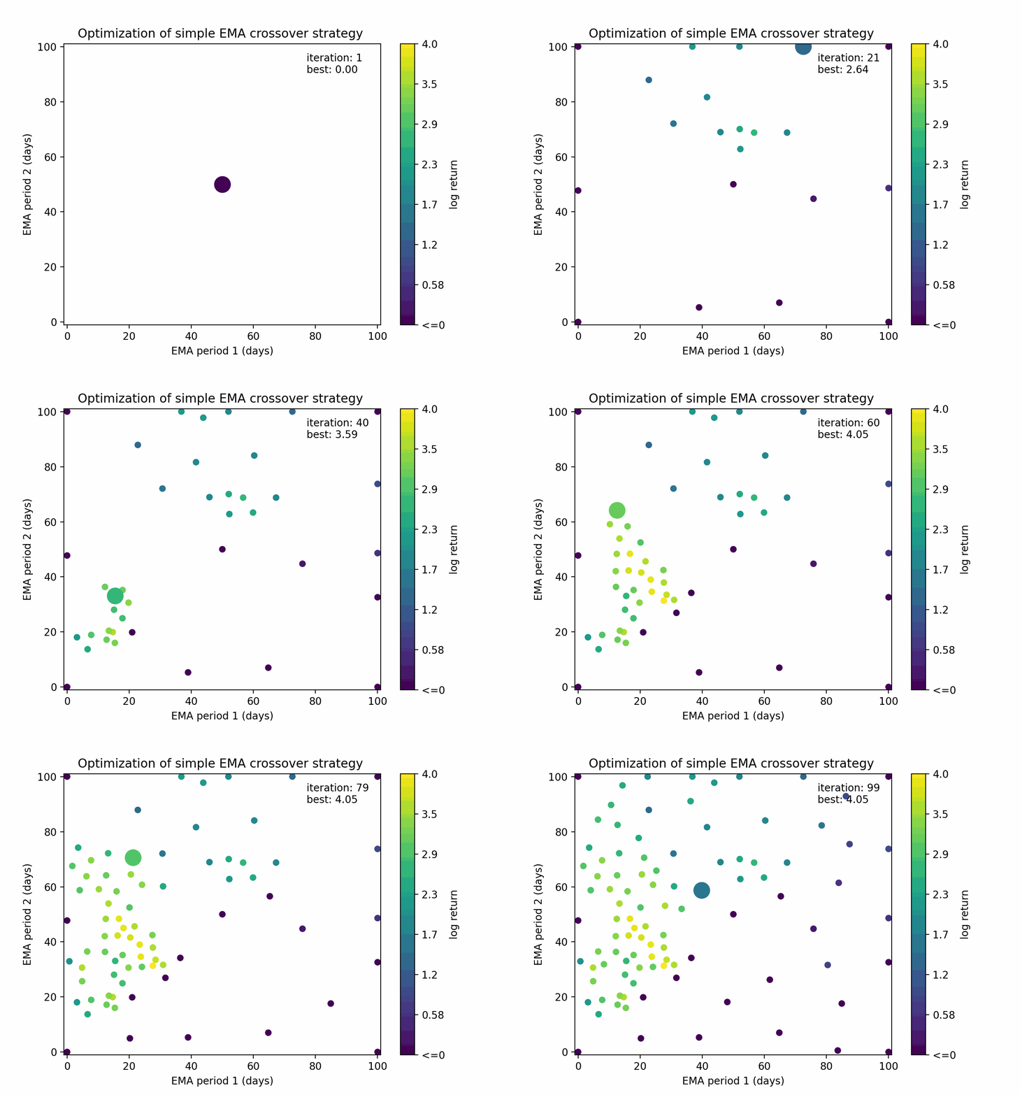
You can see that the algorithm is able to both guess points that are close to the current best solution and to explore new areas.

In summary, the main advantages of Bayesian optimization are:

• It’s parsimonious with respect to the number of function evaluations.
• It doesn’t need any assumption on the objective function.
• It’s sound, since it’s based on logic (“probabilistic” logic).
• It’s customizable (probabilistic model, acquisition function).

While the main disadvantages are:

• It could need manual tuning.
• Gaussian processes are not suited for large dimensions (more than ~10).
• Gaussian processes don’t scale well with respect to the number of observations.
• It’s probably not useful when evaluation of f(•) is not expensive.

So, Bayesian optimization is ideal when dealing with objective functions that are expensive to evaluate, where the number of parameters is relatively small and you don’t want to assume anything about the objective function. These conditions are often encountered in trading strategies.

Computational Considerations

How expensive is it to optimize a trading strategy? It depends both on the speed of the backtest and on the speed of the optimizer.

For most optimizers, the computation of the next point to evaluate takes an irrelevant amount of time with respect to a single backtest. So the bottleneck of optimization is almost always the backtest. Nevertheless, if your backtester is fast enough, you can choose to avoid parsimonious methods like Bayesian optimization, which trade the number of function evaluations with computation time for the next point to evaluate.

Conclusion

We’ve now seen how to optimize the parameters of a strategy in order to maximize the performance of a backtest, with a focus on two must-know optimizers.

This answers our second question, which is still quite different from the original one. Still unanswered is the following: Does a good backtest imply a good performance of the strategy on unseen scenarios? In general, this is not the case, so we have to put a lot of attention into several aspects in order to achieve this and avoid overfitting.

The topic of overfitting is quite fundamental and it deserves its own article, but we can still anticipate some ways that you can improve the significance of your strategy:

• Data: test your strategy on different scenarios (bull market, bear market, sideways market).
• Parameters: keep the number of parameters you optimize small; the more parameters you include, the more data you need.
• Validation: test your strategy on unseen data, whenever possible with multiple train-test splits (check out walk forward optimization).

At Trality we are working on providing optimization tools in our platform that will help users achieve better results in their backtests, so stay tuned for the next updates!